QPSeeker

QPSeeker is an end-to-end a neural database planner, encapsulating the information of the data and the given workload to learn the distributions of cardinalities, costs and execution times of the query plan space. At inference, when a query is submitted to the database, QPSeeker uses its learned cost model and traverses the query plan space using Monte Carlo Tree Search to provide an execution plan for the query.

In QPSeeker’s core is a model that learns to approximate the distributions of the cardinality, computational cost and runtime of the plans in the workload. Our approach assumes that queries with similar characteristics (e.g., number of tables, number of joins, filters applied, etc.) and complexity in terms of execution time will be close to each other in a latent space, and we use variational inference to learn this space. Hence, at the heart of our system lies a Variational Autoencoder (VAE), whose latent space is enforced to follow a Gaussian structure, where each latent dimension represents a latent feature of the data. At the end of training, similar queries and, particularly, similar query execution plans will fall close to each other in the learned latent space.

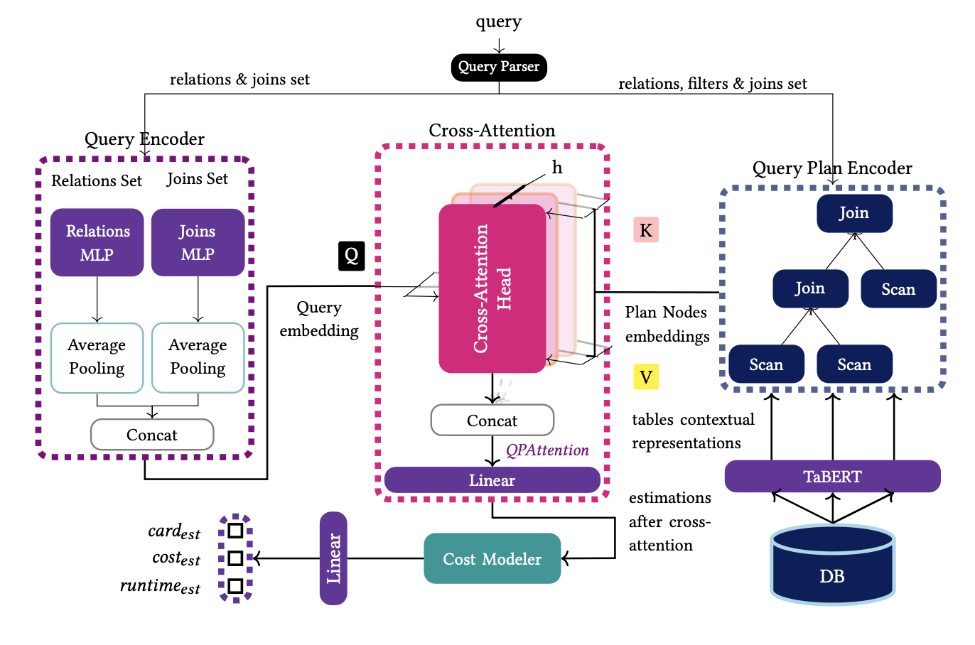
Query Encoder

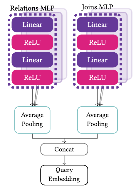
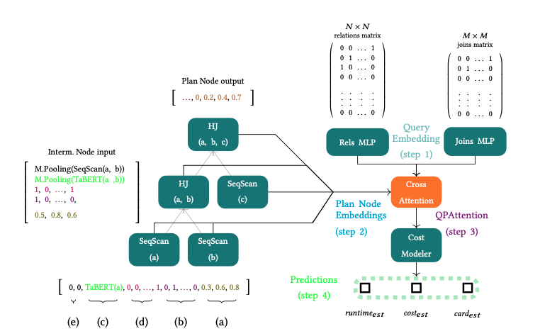
The query encoder is responsible for providing a rich representαtion of the query. Its output will be used to compute the association between the query and the execution plan. Each relation in T_q is mapped to a one-hot vector of size 𝑁 , where 𝑁 is the number of database relations. Similarly, each join in J_q is transformed into a one-hot vector with length 𝑀 equal to the number of all possible joins in the database. Each matrix, along with a column vector that serves as mask to filter the non-zero rows, into a feed forward network with five hidden layers (i.e., a Multi-layer Perceptron, MLP). Finally, the encoder applies mean pooling among the elements of each set to derive one representation for each set and concatenates the two representations to form the query embedding vector.

Plan Encoder

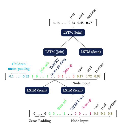
The plan encoder aims at capturing the result of the interactions of the physical operators over the tables learning from the operators and the structure of each query plan. Based on the type of the node we provide the following input per node:

Leaf Node (Scans)

Intermediate Node (Joins)

The output of each node is a vector holding information about the interaction between plan nodes and the last three dimensions are the estimations of the cardinality, cost, latency of the node in the plan.

QPAttention

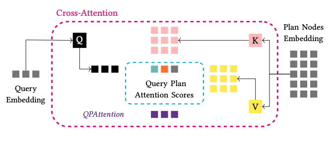
Each node does not have the same impact on the plan in terms of the execution time and computational cost for the complete plan. For example, the selection of an operator requiring more memory and hence more computational cost, like a Hash Join, will have a higher value for its cost, than an Index Scan. Therefore, we desire to give a score to each plan node and measure which nodes in the plan have the higher impact on the final estimations. To this direction, we make use of cross-attention between the query and the output of each node in the plan. For the implementation of cross-attention, we follow the standard notation and create three matrices, the query, key and value, (QKV), which are used as projection matrices for each QEP.

Cost Modeler (VAE)

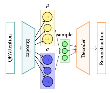
Our goal is to capture the distributions of the cardinalities, costs and execution times for the plans in the space of a query, and to generalise for the entire workload. For this purpose, at the heart of QPSeeker lies a variational autoencoder, acting as the cost modeler. The objective of the cost modeler is not only to approximate the target distributions but also to be able to generalise on unseen queries, by providing accurate estimates for each plan node statistics, and consequently, for a whole execution plan suggested by QPSeeker, through variational inference. Our belief is that execution plans with analogous complexity, in terms of runtime and execution cost, or with similar characteristics, such as relations and filters applied, if projected to a structured latent space, will have representations close to each other, depicting these similarities. The use of the VAE aims at the formation of such a latent space.

Running Example

For example, in our training set exists a 𝑄𝐸𝑃 containing the following query and execution plan:

Q: select * from a, b, c where a.a1=b.b1 and b.b2=c.c1 and a.a2>1

Plan: 1.[SeqScan(a),0.3,0.6,0,8], 2.[SeqScan(b),0.2,0.4,0.1] 3.[HashJoin(a, b),0.5,0.8,0.6], 4.[SeqScan(c),0.3,0.7,0.8] 5.[HashJoin(a, b, c),0.4,0.6,0.9]

Query Encoder takes as input the relation and join matrices and produces the query embedding vector (step 1). Then, we encode each execution plan, and we apply the cross-attention mechanism to create the input for the cost modeler. For each QEP, we get the base table representations from TaBERT and construct the input of each node. The input of each node is passed through the Plan Encoder resulting to the embedding vector of each node (step 2). The next step is the calculation of QPAttention between the query embedding and the five nodes in the plan (step 3). Then, we pass this joint embedding vector of the QEP to the variational autoencoder, and finally, (step 4) we pass the reconstructed vector into a dense layer to get the prediction for the cardinalities, costs and latencies of the encoded QEP.

After training the cost model of QPSeeker, the planner can be used for planning new queries. In order to traverse the search space fast and find a good execution plan, we use the Monte Carlo Tree Search (MCTS) algorithm. In its basis, MCTS uses randomness to select the next plan operator using sampling, thus it can estimate a near optimal action in current state with low computation effort. We use vanilla MCTS to traverse the query plan space in a bottom-up fashion. We start from base relations and apply one join at a time until all relations are present in the final plan. As a reward function, we use the Upper Confidence bounds for Trees (UCT) formula proposed be the authors:

where for the 𝑖-th node, t_i is its reward and calculates how many times the node is present in the best plan so far during the simulations. Next, n_i is the number of rollouts, t is the number of rollouts of the parent node, and C is the exploration coefficient parameter, ranging between [0, 1].

For the evaluation of each plan node, we use QPSeeker’s internal cost model. Finally, the execution plan with the least estimated execution time is considered the best plan. The reward for each node being present in the best plan discovered so far in the simulation is one unit. MCTS consists of four steps:

1. Selection

   Based on the current state of the selected subplan, the agent chooses the new plan operator in the plan with highest value, based on our policy, forming the new state of the plan.

2. Expansion

   The agent generates all possible nodes of the query plan, based on the previously selected action in the plan.

3. Rollout

   We start a simulation from the current state of the plan by randomly selecting the next operator to be applied, until the plan is complete.

4. Backpropagation

   Based on the played simulation, we estimate the execution time of the simulated plan using QPSeeker’s cost model and update the rewards.